Module 7 90 min

The single-factor model

Regress every stock on the market, and rebuild the covariance matrix from 163 numbers instead of 3,321.

Remember the uncomfortable number from Module 3: 3,321 parameters estimated from 1,114 observations. This module is the first way out.

The idea

Suppose every stock moves for two reasons: the market moved, and something happened to that company. In equation form:

r_i,t = α_i + β_i r_m,t + ε_i,t

If the εs are independent across stocks, meaning everything they have in common is captured by the market, then the covariance between any two stocks has a simple form:

Σ_ij = β_i β_j σ_m² (i ≠ j)

Σ_ii = β_i² σ_m² + σ_εi²

Or in matrix form:

Σ = ββ′ σ_m² + D

Count the parameters: 81 betas, 81 residual variances, one market variance. 163 numbers instead of 3,321. That is the main argument for factor models.

Step 1: choose the market series

Use CUKX.L, the accumulating ETF (see Module 1). Regressing dividend-inclusive stock returns on a dividend-free index biases your alphas down by roughly the yield.

Compute weekly market returns the same Wednesday-to-Wednesday way.

Step 2: run 81 regressions

The easy way

For each stock you need the slope, the residual volatility and R²:

beta       =SLOPE(ReturnsW!B2:B1115, Mkt!B2:B1115)
alpha      =INTERCEPT(ReturnsW!B2:B1115, Mkt!B2:B1115)
r-squared  =RSQ(ReturnsW!B2:B1115, Mkt!B2:B1115)
resid vol  =STEYX(ReturnsW!B2:B1115, Mkt!B2:B1115)

STEYX is the standard error of the regression, which is the residual volatility you want, already using the n−2 denominator.

Lay these out as four rows above your return block and drag across. That is 81 regressions from four formulas.

Or do it as matrix algebra

LINEST(y_range, x_range) returns slope and intercept together, and the full statistics if you pass TRUE as the fourth argument. If you want to see the normal equations explicitly — β = (X′X)⁻¹X′y — MINVERSE and MMULT will do it, and it is a useful exercise.

Step 3: rebuild the matrix

=MMULT(betas, TRANSPOSE(betas)) * MktVar

then add residual variances down the diagonal only.

Now compute your portfolio volatility with this Σ instead of the sample one.

What you should find

The two numbers will be close but not equal, typically within a percentage point or so.

The differences are informative. The single-factor model assumes all correlation runs through the market. But the large miners move together for reasons that have nothing to do with the FTSE 100, and so do the banks. The model cannot see that, so it understates risk for a portfolio concentrated in one sector and is roughly right for a well-spread one.

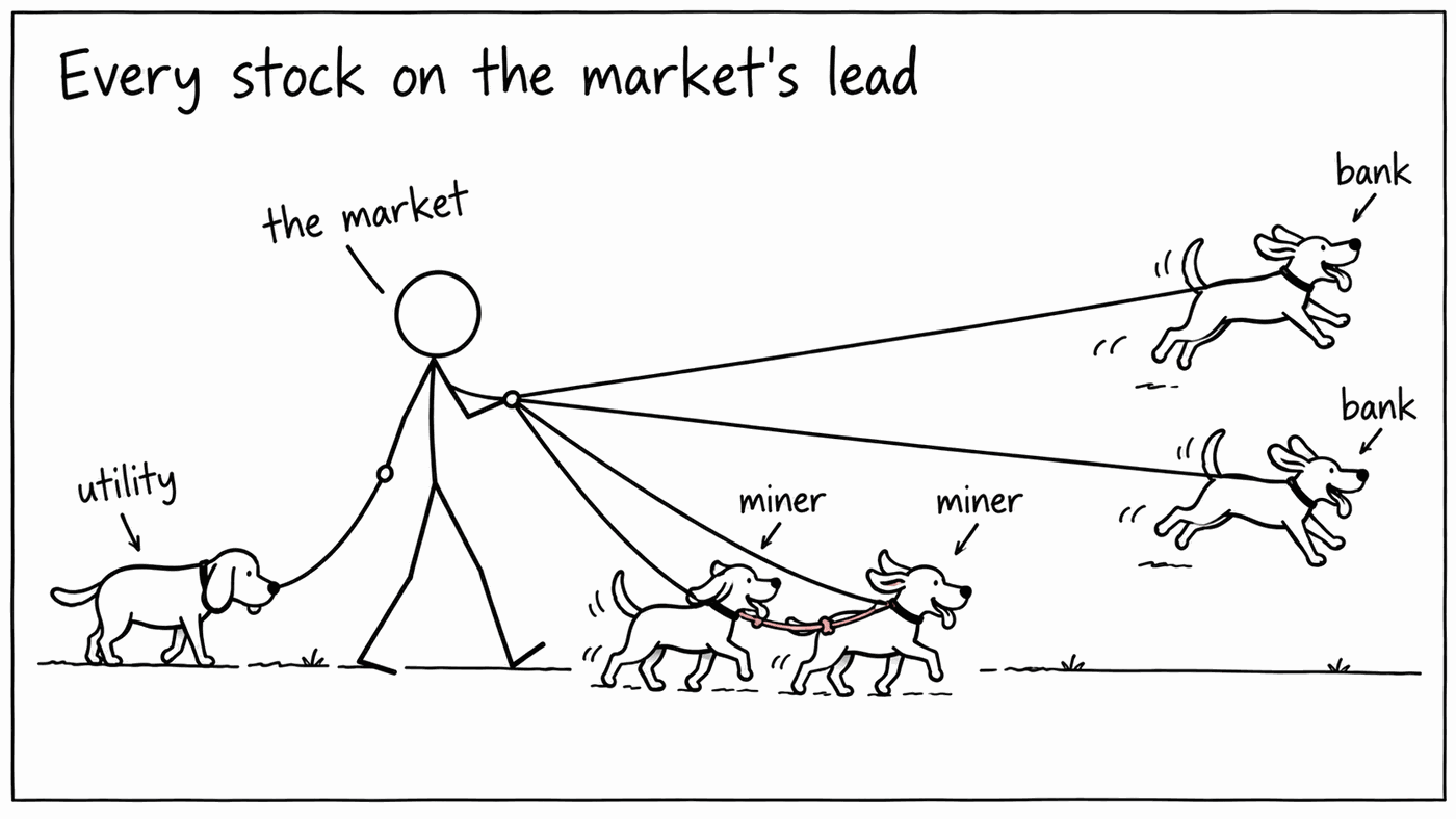
A cartoon titled Every stock on the market's lead. A stick figure labelled the market walks five dogs. Two labelled bank bound far ahead on long taut leads, one labelled utility plods behind on a short slack lead, and two labelled miner trot side by side, tied to each other by a pink rope the walker has not noticed. — The single-factor model sees each stock's lead to the market and nothing else. The miners are also tied to each other, and the model cannot see that.

Test it. Build equally-weighted portfolios of five banks, five miners, five utilities, and then five names from five different industries. Compare the single-factor prediction against what each actually realised:

Portfolio	Realised	Single-factor	Error
Five banks	24.7%	21.0%	−3.7pp
Five miners	32.5%	25.5%	−7.0pp
Five utilities	19.1%	13.9%	−5.2pp
One per industry	17.2%	18.1%	+0.9pp

Every concentrated portfolio is understated, and the well-spread one is close. This is the typical weakness of a single-factor model: the error is largest for concentrated portfolios, which are often the ones people ask about.

Module 8 addresses part of this.

Bias versus variance

Neither number is exact. The sample matrix fits the past closely, including the noise. The factor model imposes structure that is partly wrong but estimated much more precisely. This is the bias-variance trade-off, which comes up throughout risk modelling.

In practice the factor model often forecasts better out of sample, despite being a worse description of the past. This is counter-intuitive, and it matters in practice.

Things to look at

Beta distribution. Banks and miners well above 1, staples and utilities below. Does the ranking match your intuition?
R². Typically 0.2–0.5 here, so the market explains under half the variance of a typical stock. The rest is specific risk.
Beta is unstable. Compute it over 2005–2007, then 2008–2010. Bank betas change a great deal. Beta is an estimate that changes over time.
Portfolio beta. The weighted average of your holdings' betas tells you how much of your risk is simply market exposure.

Check your answers

← Value at Risk

The cross-sectional factor model →