Module 6 75 min

Value at Risk

Parametric VaR is one formula. Historical VaR makes fewer assumptions. Then test whether either one worked.

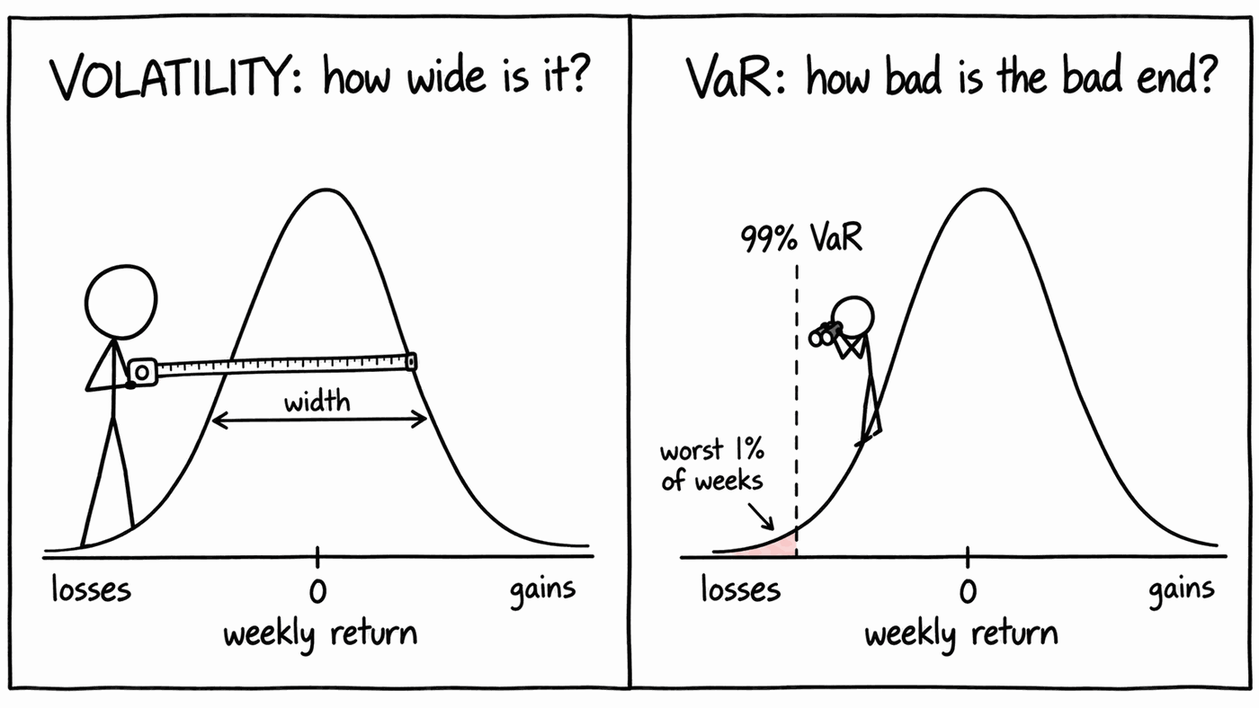
Volatility describes the whole distribution. VaR asks a narrower question: how bad is a bad week?

VaR at 99% over one week is the loss that should be exceeded in only 1 week in 100.

Two cartoon panels. Left, titled Volatility: how wide is it? A bell curve of weekly returns with a stick figure measuring its width with a tape measure. Right, titled VaR: how bad is the bad end? The same curve with a dashed line far out on the losses side marked 99% VaR, the small shaded tail beyond it labelled worst 1% of weeks, and a worried stick figure peering at it through binoculars. — Volatility measures how spread out the whole distribution is. VaR only cares about one point far out in the loss tail.

Parametric VaR

Assume returns are normal. Then the 99th percentile is 2.326 standard deviations below the mean, and:

VaR_99% = −(μ × h + z_0.01 × σ × √h)

With μ set to zero over a one-week horizon (the estimate is mostly noise at this horizon), this reduces to 2.326 × the weekly volatility.

One cell

=-NORM.S.INV(0.01) * SQRT(PVar)

NORM.S.INV(0.01) is −2.326, so the minus sign gives a positive loss. Note SQRT(PVar) is the weekly volatility — do not annualise first. Scaling a one-week VaR to ten days uses the same √T rule, and relies on the same iid assumption discussed in Module 2.

Historical VaR: the honest one

Historical VaR makes no distributional assumption and uses the portfolio's own history.

Compute your portfolio's realised return for every week: =MMULT(ReturnsW!B2:M1115, weights) — one number per week.
Take the 1st percentile of that series.

One cell again

=-PERCENTILE.INC(PortRet, 0.01)

Use PERCENTILE.INC for consistency with the answer key. PERCENTILE.EXC interpolates differently in the tails and will put you outside tolerance.

Compare them

Historical VaR will come out larger than parametric, typically by 15–25% on this data.

The gap reflects the fat left tail of equity returns: extreme moves happen more often than a normal distribution predicts. The normal distribution says a −5% week should occur about once a decade. Count them in your own series.

Historical VaR has its own problem

It cannot produce a loss bigger than the worst one in your sample. Estimated on 2004–2007 data, historical VaR would have put the worst week at about −6%. It also weights a week from 2009 exactly as heavily as last week, which is the window problem from Module 5, back again. A common fix is to EWMA-weight the historical observations.

Expected shortfall

VaR gives the threshold but says nothing about losses beyond it. Expected shortfall (conditional VaR) is the average loss given that you breached:

=-AVERAGEIF(PortRet, "<"&PERCENTILE.INC(PortRet,0.01))

It is typically 1.3–1.6× the VaR. Regulators have largely moved to ES, partly because VaR says nothing about the size of losses beyond the threshold, and partly because VaR is not sub-additive: the VaR of a combined book can exceed the sum of its parts, which is absurd for a risk measure. ES does not have that problem.

Options: the simplest reason to revalue

Everything so far has been a portfolio of shares, whose value moves in a straight line with the prices. Plenty of portfolios hold something that does not. Options are the obvious example; convertible bonds and structured products are others.

Parametric VaR can only handle an option by approximating it with its delta: the number of units of the underlying it behaves like for a small move. That is accurate for small moves and increasingly wrong for large ones, and large moves are what VaR is about.

Historical VaR has no such problem. Reprice the option under each historical move and take the percentile of the profits and losses that result. This is called full revaluation. Monte Carlo does the same thing with simulated moves.

Here is how much it matters. Take the benchmark at 100, one-month options priced at the benchmark's own volatility of 17.1%, zero interest rates, and a one-week horizon. The 99% one-week VaR, in index points:

Position	Delta-normal	Normal moves, full revaluation	Historical moves, full revaluation	Worst week in the sample
The index alone	5.52	5.52	6.82	−13.89
Short an at-the-money put	2.71	3.78	5.00	−12.00
Short a put 5% out of the money	0.74	1.50	2.29	−8.57
The index plus a long at-the-money put	2.81	1.74	1.82	−1.89

The middle column still assumes normal returns but reprices the option properly, so the step from the first column to the second is purely the option's curvature. The step from the second to the third is the fat tail, as in the index-alone row.

Short puts are understated. For the out-of-the-money put, delta-normal VaR is 0.74. Curvature alone doubles it, and fat tails take it to 2.29. The seller collected a premium of 0.33, and the worst week in the sample cost 8.57.
Protective puts are overstated. The put puts a floor under the loss, and the worst week cost 1.89, barely more than the put's price. Delta-normal cannot see the floor and reports 2.81, half as much again as the full-revaluation answer.

The mechanism is gamma, the rate at which delta changes. A short option loses faster and faster as the market moves against it; a long option loses more and more slowly. A delta-gamma approximation adds that second-order term, and gets much closer (3.99 and 1.44 for the two short puts), but full revaluation is the straightforward answer whenever you can reprice the position.

Repricing a put under every historical week

Black–Scholes with zero rates, for spot S, strike K, years to expiry T and volatility v:

d1    =(LN(S/K) + 0.5*v^2*T) / (v*SQRT(T))
d2    =d1 - v*SQRT(T)
put   =K*NORM.S.DIST(-d2, TRUE) - S*NORM.S.DIST(-d1, TRUE)
delta =NORM.S.DIST(d1, TRUE) - 1

Price the put today with S = 100 and T = 4/52. Then, for each historical weekly return r, reprice it with S = 100 × (1 + r) and T = 3/52. For a short put the week's P&L is today's price minus the new one. The VaR is -PERCENTILE.INC of that column at 0.01, exactly as before.

The table flatters the short puts

It holds implied volatility fixed at 17.1%. In a real sell-off implied volatility jumps, which makes a short put lose more still. A proper full revaluation moves the volatility as well as the price.

Backtesting

A VaR number is a prediction, so it can be tested against what happened.

At 99% over 1,114 weeks you expect about 11 exceptions. Count your actual ones:

=COUNTIF(PortRet, "<"&-VaR)

Too many and you are understating risk. Too few and you are holding capital against losses that do not happen.

The Kupiec test

Is your exception count statistically plausible? The proportion-of-failures test:

LR = −2 ln[ (1−p)^n−x p^x ] + 2 ln[ (1−x/n)^n−x (x/n)^x ]

with n observations, x exceptions and p = 0.01. Under the null that your model is calibrated, LR follows χ² with one degree of freedom. Reject at 95% if LR > 3.841.

=CHISQ.DIST.RT(LR, 1)

What Kupiec misses

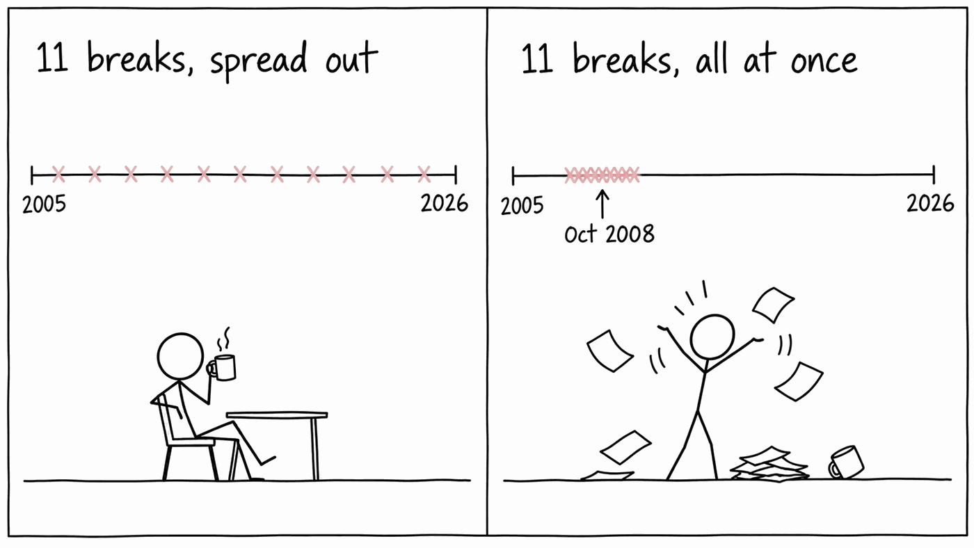
It counts exceptions but ignores when they happened. Eleven exceptions spread evenly over twenty years suggests a reasonable model; eleven exceptions all in October 2008 suggests a model that failed in the period that mattered most. The Christoffersen test adds a clustering check, and in practice clustering is often the more serious problem.

Two cartoon panels, each with a timeline from 2005 to 2026. Left, titled 11 breaks, spread out: pink crosses evenly spaced along the whole line, and a relaxed stick figure sipping tea. Right, titled 11 breaks, all at once: the pink crosses crammed together at Oct 2008, and a stick figure flailing as papers fly. — Kupiec counts the breaks, so it rates these two models the same. The one on the right failed in the one month that mattered.

In practice: the UCITS rule of thumb

Regular backtesting of VaR breaks is a regulatory requirement for UCITS funds in Europe that measure global exposure using VaR. The CESR guidelines (CESR/10-788) keep it simple. Count the days in the most recent 250 business days, roughly a year, on which the one-day loss exceeded the one-day 99% VaR. A well-calibrated model should produce about 2.5. If there are more than four, senior management, and the regulator where applicable, must be told at least quarterly, with an analysis of what caused the breaks and what was done about it.

So in practice the Kupiec test is replaced by a much simpler rule of thumb. The two are worth comparing, using the Kupiec formula above with 250 days:

Breaks in 250 days	Kupiec p-value	Rejected at 95%?	Chance of at least this many if the model is right
4	0.38	No	24%
5	0.16	No	11%
6	0.06	No	4%
7	0.02	Yes	1%

The rule of thumb is stricter than Kupiec. Five breaks is nowhere near a statistical rejection, but it still triggers an investigation, so roughly one correctly calibrated fund in nine will trip it in a given year through bad luck alone. That is a sensible trade for a regulator, who would rather look into a few false alarms than miss a broken model, and worth remembering when you are the one writing the explanation.

The threshold of four matches the edge of the green zone in the Basel traffic-light test for bank trading books, where five to nine breaks in 250 days is amber and ten or more is red.

Daily versus weekly

The regulatory count uses one-day VaR and daily profit and loss. The backtest in this module uses weekly returns over the whole sample, so the two sets of numbers are not directly comparable. To apply the rule yourself, rerun the backtest on daily returns for the most recent 250 business days.

Run the backtest on both your parametric and your historical VaR. One of them will do noticeably better. Form a view on why.

Check your answers

← Time windows and exponential weighting

The single-factor model →