Module 3 90 min

The covariance matrix

Build the whole matrix in one formula, then squeeze it with a weight vector to get portfolio volatility.

This module is the centre of the exercise; the later modules build on it.

Why covariance

A covariance between two sets of returns captures both how much each varies by itself, and the correlation between them. In fact you can define a covariance exactly that way:

σ_ij = σ_i × σ_j × ρ_ij

the product of each stock's standard deviation and the correlation between them — a number running from −1 to +1, representing how much they move with respect to each other.

So it is a handy portmanteau measure for each pair, capturing three separate bits of information in one number. On the diagonal, where a stock is paired with itself, the correlation is 1, so the covariance is σ_i², the plain variance.

Once you have this for every possible pair of stocks, you have basically captured everything — almost everything, until we move away from Normal land — about the risk of any combination of these stocks.

In a sense, all a risk model is is a covariance matrix, calculated in some way. Modules 5, 7, 8 and 9 are four different ways of calculating one. Each ends in a covariance matrix; they differ in how it is estimated.

And the way to retrieve a single risk number from the model is to multiply your chosen portfolio weights by the covariance matrix. Although, as you will see, you actually multiply by the weights twice — once vertically and once horizontally.

What you are building

For N stocks, Σ is an N×N matrix where the entry in row i, column j is the covariance between stock i and stock j. The diagonal holds each stock's variance.

With 81 names that is 6,561 cells, or 3,321 distinct numbers, so you will not want to type a formula for each one.

The quick way: a grid of `COVARIANCE.S`

Lay your tickers down column A and across row 1 of a Cov sheet, then fill the grid with one covariance per pair. Each cell holds the covariance between that row's stock and that column's stock.

It is 6,561 cells for 81 names and recalculates more slowly than the matrix version. It works, and it earns the same marks.

The art is in getting each cell to point at the right two columns of returns without typing 6,561 different ranges. There are a few ways, and the team is split on which is best:

Pointing each cell at the right columns

Assume weekly returns in ReturnsW!B2:CD1115 (1,114 weeks, 81 stocks), tickers in ReturnsW!B1:CD1, and your Cov grid starting at B2 with the same tickers, in the same order, down column A and across row 1.

OFFSET, moving across by the row and column number of the cell you are in:

=COVARIANCE.S(OFFSET(ReturnsW!$A$2, 0, ROW()-1, 1114, 1),
              OFFSET(ReturnsW!$A$2, 0, COLUMN()-1, 1114, 1))

INDIRECT, building each range as a text address. It shows clearly what it is doing, but it is the most tedious to type:

=COVARIANCE.S(INDIRECT("ReturnsW!" & ADDRESS(2, ROW(), 4) & ":" & ADDRESS(1115, ROW(), 4)),
              INDIRECT("ReturnsW!" & ADDRESS(2, COLUMN(), 4) & ":" & ADDRESS(1115, COLUMN(), 4)))

INDEX with MATCH, looking each column up by ticker. An INDEX row argument of 0 returns the whole column:

=COVARIANCE.S(INDEX(ReturnsW!$B$2:$CD$1115, 0, MATCH($A2, ReturnsW!$B$1:$CD$1, 0)),
              INDEX(ReturnsW!$B$2:$CD$1115, 0, MATCH(B$1, ReturnsW!$B$1:$CD$1, 0)))

This one matches on the ticker name rather than on position, so it still works if someone re-sorts the columns.

Write one cell, then drag across and down.

OFFSET and INDIRECT are volatile

Both recalculate every time anything in the workbook changes, not just when their inputs do. Across 6,561 cells that is noticeable. To avoid slow recalculation, switch to manual (Formulas → Calculation Options) and press F9 when you want fresh numbers. INDEX is not volatile.

COVAR is not COVARIANCE.S

If you use the old COVAR function, note that it is the population covariance, dividing by n rather than n−1 — the same as COVARIANCE.P.

This is the opposite of STDEV in Module 2, which defaults to the sample version, so the two legacy functions are inconsistent with each other.

With 1,114 weekly observations the difference is a factor of 1114/1113 on the variance, about 0.045% on the volatility. That is comfortably inside the checker's tolerance, so COVAR still gets full marks. It does mean the diagonal of your grid will be very slightly below the VAR.S of each column.

Before you commit to the quick way

It works perfectly well for this module. But in Module 5 you will be asked to weight recent weeks more heavily than old ones, and COVARIANCE.S has no way of doing that — every observation counts equally, and there is no weights argument to slip in. You would be rebuilding the whole grid, and you are really going to wish you had built it the pure way.

The pure way below writes the covariance matrix as R′R. Once it is in that form, weighting the observations is just a matter of scaling each row of returns by the square root of its weight before the same MMULT: one extra column, and nothing else changes.

The pure way: seeing the guts of the calculation

This route shows how the covariance matrix is built. It is worth doing at least once, even if you build your model the quick way, because Module 5's exponential weighting and Module 9's principal components are much easier to follow, and to build, once you see the covariance matrix as matrix algebra.

Take your weekly returns as a matrix R with T rows (dates) and N columns (stocks). Subtract each column's mean, so every column is centred on zero. Then:

Σ = R′R / (T − 1)

The (i,j) entry of R′R is the sum over all dates of r_i,t × r_j,t. Since the columns are demeaned, that sum divided by T−1 is exactly the sample covariance — the same number COVARIANCE.S gives you for that pair. The matrix product computes all 3,321 of them at once.

Doing it in Excel

With weekly returns in ReturnsW!B2:CD1115 (T = 1,114 rows, N = 81 columns):

Step 1 — demean. Put each column's mean in row 1 of a new Dev sheet, above where its demeaned returns will go:

=AVERAGE(ReturnsW!B2:B1115)

then in Dev!B2, and dragged across and down:

=ReturnsW!B2 - B$1

Unglamorous and reliable. On a 365 build you can do the whole block in one spilled formula instead:

=ReturnsW!B2:CD1115 - BYCOL(ReturnsW!B2:CD1115, LAMBDA(c, AVERAGE(c)))

Step 2 — the matrix. On a Cov sheet, in one cell:

=MMULT(TRANSPOSE(Dev!B2:CD1115), Dev!B2:CD1115) / (COUNT(Dev!B2:B1115) - 1)

On Microsoft 365 this spills into an 81×81 block automatically. Label the rows and columns with your tickers — you will regret it if you do not.

If you built the quick way as well, subtract one grid from the other. Every cell should be zero, or within floating-point noise of it.

Performance

That multiply is 1,114 × 81 × 81 ≈ 7.3 million operations, and Excel redoes it on every recalculation. If the sheet becomes sluggish, switch to manual calculation and press F9 when you want it. This is also why we suggest weekly rather than daily returns for the full-universe matrix: daily would be five times the work for a noisier answer.

Sanity checks

Each of these catches a common bug.

Symmetry. Σ_ij must equal Σ_ji. Check a few pairs, or =SUMPRODUCT(ABS(Cov-TRANSPOSE(Cov))) should be ~0.
The diagonal is variance. SQRT of a diagonal entry, times √52, must match the annualised vol you computed in Module 2 for that stock.
Correlations are in range. Σ_ij / (σ_iσ_j) must lie in [−1, 1]. A value outside that range usually means misaligned rows, from a stray blank or an off-by-one.
Everything is positive. Every diagonal entry. A negative variance means you have blanks being read as zeros.

Blank cells

A blank cell in a return block is treated as zero, not as missing. A stock that did not trade looks like a stock that did not move, which drags its variance and every one of its covariances toward zero. If one name looks implausibly calm, look for gaps.

Portfolio volatility

Now the payoff. With a weight vector w:

σ_p² = w′Σw σ_p = √(w′Σw) × √52

A cartoon titled Squeeze the matrix with the weights. A row vector labelled w prime, a square grid labelled Sigma and a column vector labelled w sit clamped in a bench vice. A stick figure heaves on the handle, and a single small pink square labelled portfolio variance has dropped out underneath. — Multiply by the weights once across and once down, and the whole covariance matrix squashes into a single number: the portfolio's variance.

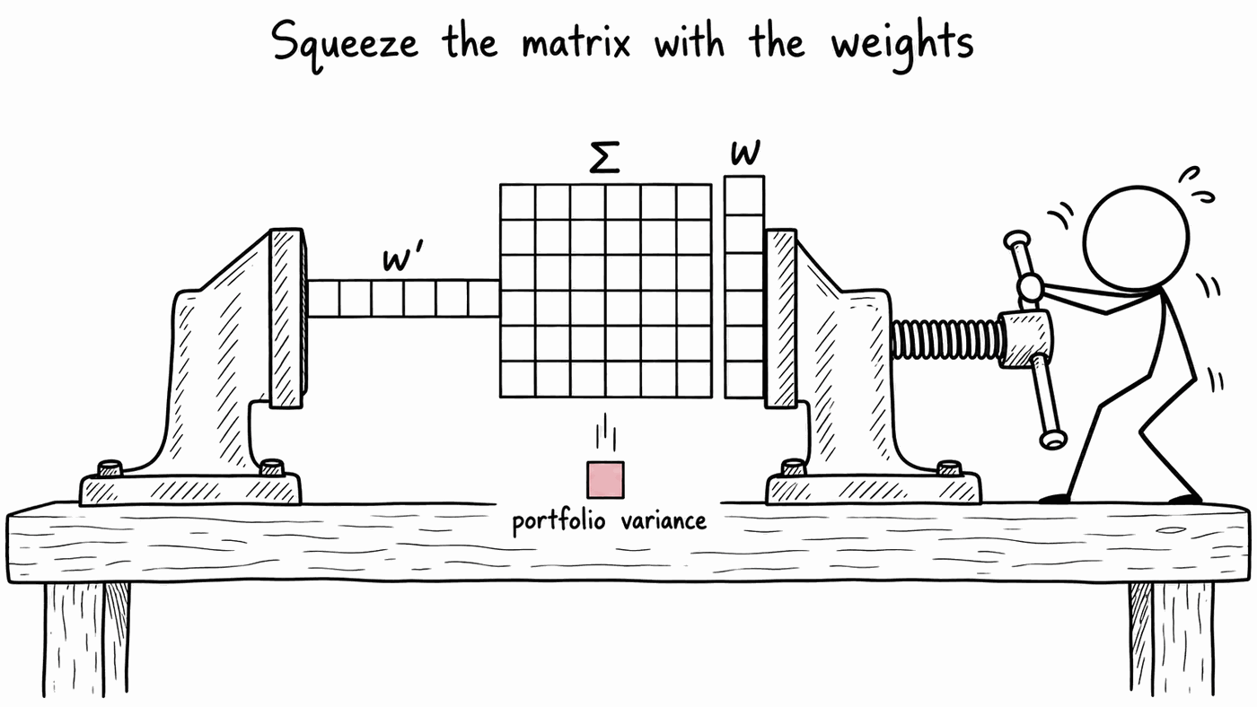
The front tab

Build a sheet with your tickers down column A and your weights in column B. Then, in a single cell:

=SQRT(MMULT(MMULT(TRANSPOSE(B2:B13), Cov!B2:M13), B2:B13)) * SQRT(52)

Two nested MMULTs: the inner one gives Σw, the outer one gives w′(Σw). Both return a 1×1 result, so SQRT can be applied directly.

Make sure your weight order matches your covariance row order exactly. A mismatch produces a plausible-looking wrong answer rather than an error, so it is easy to miss.

If you would rather avoid MMULT entirely:

=SQRT(SUMPRODUCT(Cov!B2:M13, MMULT(B2:B13, TRANSPOSE(B2:B13)))) * SQRT(52)

or build the full grid of w_iw_jΣ_ij on a tab and sum it. All three give the same number.

What you should notice

Your portfolio's volatility should come out below the weighted average of the individual stock volatilities. That gap is diversification, often called the only free lunch in finance. Compute both and look at the difference.

Then set one weight to 100% and the rest to zero. You should get that stock's own volatility back. If you do not, the weights and the matrix are misaligned.

A number to consider

You estimated 3,321 parameters from 1,114 observations, which is about three times as many unknowns as data points.

The matrix is still valid (it is positive semi-definite by construction, because R′R always is), but a good part of it is estimation noise dressed up as correlation. Modules 7, 8 and 9 are three different escapes from that problem.

Check your answers

← Returns, and the square root of time

Tracking error and where the risk comes from →