Module 2 60 min

Returns, and the square root of time

Three frequencies, log versus simple, and why annualising daily vol does not quite match annualising monthly vol.

This module starts the calculations. You are going to build three return series from one price series, annualise all three, and then look at why they disagree.

The file you need from here on

Work from the core workbook — 81 names, 2005 onwards, already screened and trimmed to a complete rectangle with no gaps.

This is the same data you were working with in Module 1, after the decisions you just made have been applied. Everyone uses this file from now on, so that everyone's numbers agree.

Simple or log?

simple: r_t = P_t / P_t-1 − 1 log: r_t = ln(P_t / P_t-1)

Both are defensible. The rule of thumb on this desk:

Log returns add up across time. Twelve monthly log returns sum to the annual log return. They are what you want for compounding, and they are symmetric: −50% then +100% nets to zero.
Simple returns add up across assets. A portfolio's simple return is the weighted sum of its holdings' simple returns. Log returns do not have this property — the log return of a portfolio is not the weighted average of log returns.

Because a covariance matrix is used together with portfolio weights, and weights combine across assets, we use simple returns throughout. Build both if you like; over daily horizons they differ in the fourth decimal place.

Doing it in Excel

With your prices in Prices!B2:CD5407, put this in the first cell of a new ReturnsD sheet and drag:

=Prices!B3/Prices!B2-1

Or, if you want the whole block in one formula on a 365 build:

=Prices!B3:CD5407/Prices!B2:CD5406-1

Label your ReturnsD tab. Two things will help avoid bugs later:

A date column down the left. You will need it for filtering to Wednesdays, cutting windows, and finding particular crises.
A top row of tickers, copied across from the Prices tab. When you later feed a returns block into a covariance matrix and then multiply by a weight vector, the columns need to be in the order you think they are, and labels let you check that.

On dates: conventionally a daily return is labelled with its end date. The return from Monday's close to Tuesday's close is Tuesday's return, because Tuesday is when you would have earned it. So your first return sits against the second date in the price file, not the first, and your ReturnsD tab has exactly one row fewer than Prices.

It is easy to end up one row out, which puts returns against the wrong dates and distorts every correlation in the model.

Weekly: use Wednesdays

Do not just take every fifth row. Sample Wednesday closing prices, then take returns of that series.

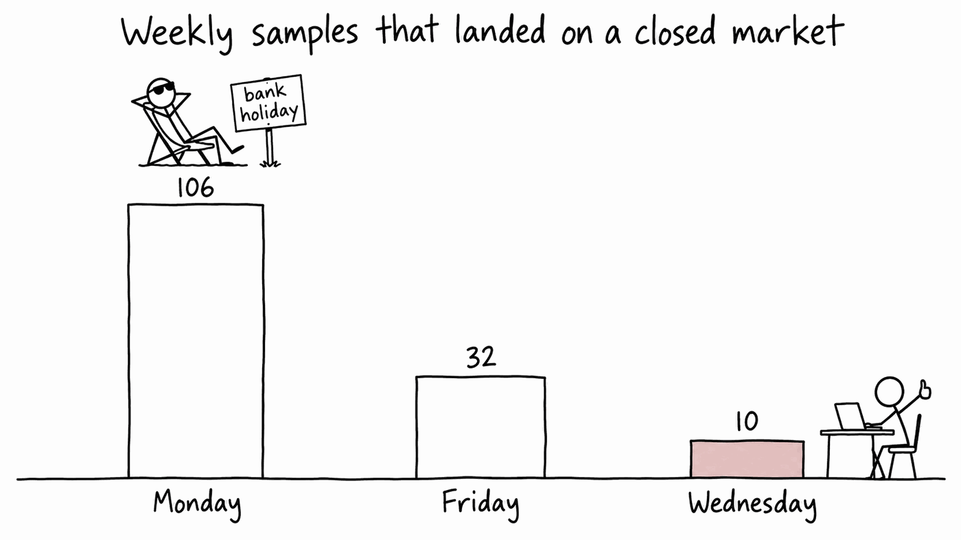
The reason is the one from Module 1: UK market holidays cluster on Mondays and Fridays — Good Friday, Easter Monday, May Day, and the spring and August bank holidays. A Friday-to-Friday week is regularly only four trading days long, which adds a seasonal error to your variance. Wednesday is the day least affected by UK holidays.

A cartoon bar chart titled Weekly samples that landed on a closed market. Monday 106, Friday 32, Wednesday 10, with the Wednesday bar shaded pink. A stick figure lounges in a deckchair on top of the Monday bar beside a bank holiday sign; another sits at a laptop next to the Wednesday bar giving a thumbs up. — How often each choice of weekday landed on a day the London Stock Exchange was shut, across this dataset.

Getting Wednesdays

Route one: filter the rows you have. Add a helper column next to your dates:

=WEEKDAY(A2,2)=3

(WEEKDAY with return-type 2 makes Monday 1, so Wednesday is 3.) Then filter to TRUE, or use FILTER:

=FILTER(A2:CD5407, WEEKDAY(A2:A5407,2)=3)

Route two: build the grid you want. Often easier. Put any Wednesday in a cell, then below it:

=A2+7

and fill down. This gives you a regular weekly calendar that does not depend on which dates appear in the price file.

Route two leaves you needing to pull a price for each of those dates, and some of them will be bank holidays with no row in the file. An approximate-match VLOOKUP handles this by snapping each grid date onto the last trading day at or before it. See Snapping a date grid onto real trading days, further down this page; it works the same way for weekly and monthly.

Monthly: use month ends

Same two routes as the weekly case.

Filter the rows you have. Flag a row when the month of the next date differs from the month of this one:

=MONTH(A3)<>MONTH(A2)

That marks the final trading day of each month. Filter on it.

Or build the grid. EOMONTH gives you calendar month ends directly — put a start date in a cell, then below it:

=EOMONTH(A2,1)

and fill down, for a series of month ends.

However, the last calendar day of a month is often not a trading day. 31 August is a bank holiday about one year in seven, and 25 December never trades. So some of the dates in your grid will have no row in the price file.

Snapping a date grid onto real trading days

This works the same way for weekly and monthly grids.

VLOOKUP with its fourth argument set to TRUE does an approximate match: on a column sorted ascending, it returns the row with the largest value less than or equal to your lookup date. That gives you the last trading day on or before the date.

With your grid dates down column A and your tickers along row 1 (the top row of tickers from earlier now earns its keep):

=VLOOKUP($A2, Prices!$A:$CD, MATCH(B$1, Prices!$A$1:$CD$1, 0), TRUE)

Drag it across and down. Each bank holiday resolves to the previous trading day, so you do not need to handle Good Friday separately.

Three things to watch for:

The lookup column must be sorted ascending. Dates in the price file are, but if you have re-sorted anything, TRUE returns confident nonsense rather than an error.
A grid date before the first row of prices gives #N/A. Start your grid inside the sample.
It always snaps backwards. A grid date after your last price returns the last price you have, rather than an error, which sets the most recent return to zero. Stop the grid at your final date.

Bonus marks if you work out XLOOKUP as well. Its fifth argument is a match mode, and -1 means "exact match, or the next smaller item" — the same snapping behaviour, without the fragile column counting:

=XLOOKUP($A2, Prices!$A:$A, Prices!B:B, , -1)

Further bonus marks for constructing some Frankenstein formula out of INDEX and MATCH instead. MATCH with a third argument of 1 is the same approximate match on its own, handing back a row number for INDEX to fetch from:

=INDEX(Prices!B:B, MATCH($A2, Prices!$A:$A, 1))

This is the route the purists prefer, on the grounds that it does not care where the lookup column sits relative to the answer. They are right, and they will tell you so.

Annualising: the square root of time

σ_annual = σ_period × √(periods per year)

With 252 trading days, 52 weeks and 12 months:

Frequency	Multiplier
Daily	√252 ≈ 15.87
Weekly	√52 ≈ 7.21
Monthly	√12 ≈ 3.46

It is the volatility that scales with √T, because variance scales with T. Variance adds up over independent periods; standard deviation does not. If you ever find yourself multiplying a volatility by 252, stop.

The calculation

=STDEV.S(ReturnsD!B2:B5406) * SQRT(252)

Use STDEV.S (sample, divides by n−1), not STDEV.P. With thousands of observations it makes little practical difference, but the sample estimator is the convention everyone else uses.

Some particularly ancient members of the team still insist on plain STDEV, which is ambiguous about which one it means. Excel quietly covers for them by defaulting it to STDEV.S, so they have got away with it for twenty-five years and see no reason whatsoever to stop now. You may form your own view on whether a function deprecated in 2010 constitutes a house style or a personality trait.

Be warned that at least one of them had a hand in writing this exercise, so expressing a strong opinion on the matter is a career decision rather than a technical one.

Now the interesting bit: why they disagree

Compute the annualised volatility of your assigned stock three ways. You will get three different numbers, typically with the daily figure highest and the monthly lowest, often by two or three percentage points.

This is expected. The √T rule assumes returns are independent and identically distributed, and real returns are not:

Negative autocorrelation at short horizons. Bid-ask bounce and over-reaction mean a down day is slightly more likely to be followed by an up day. Sum the variance over a week and the cross terms are negative, so the week is less volatile than 5 × a day. Scaling daily vol up therefore overstates weekly risk.
Volatility clustering. Calm begets calm, and crisis begets crisis, so returns are not identically distributed through time.
Fewer observations. Your monthly series has around 250 points against 5,400 daily. The standard error of a volatility estimate is roughly σ/√(2T), so the monthly estimate is noisier.

The practitioner's answer

Match the estimation frequency to your decision horizon. If you rebalance monthly, monthly returns describe your risk best, whatever the daily number says. Most equity risk models use weekly as a compromise: enough observations to estimate a large covariance matrix, and long enough to avoid most of the microstructure noise.

Run the same comparison on a high-beta bank and on a utility. The gap between daily and monthly is usually wider for the bank. Ask yourself why.

What to hand in

Three annualised volatilities for your assigned stock, below. And a one-line answer, to yourself, to: which of these three would you quote to a portfolio manager, and why?

Check your answers

← The data, and what is wrong with it

The covariance matrix →