Tracking error and where the risk comes from
Active weights, and decomposing total risk into per-holding contributions that actually add up.
On this desk the question is usually about relative risk rather than total volatility: how far can this portfolio drift from its benchmark?
Active weights
One quick adjustment to the covariance calculation swaps the answer for a relative number: just use the relative weights in the calculation, and leave the covariance matrix alone.
This will give the right total tracking error. But often the most interesting question is not what the total number is, but which holdings — or, later on, which factors — are driving it: what is the tracking error breakdown? Interestingly, just swapping in relative weights causes problems for the breakdown of risk. More on that at the end of the module.
Two useful properties:
- Active weights sum to zero. A long-only portfolio has a long/short active position, which is why tracking error can be small even when both portfolio and benchmark are volatile.
- If you hold the benchmark exactly, wa is all zeros and TE is zero. This makes a good test: set your weights equal to the benchmark weights on your front tab and confirm you get zero.
Your benchmark weights are on the home page — cap weights across your own holdings, renormalised to 100%.
What the number means
Tracking error is a one-standard-deviation annual figure. A TE of 4% means that in roughly two years out of three, your relative return should land within ±4% of the benchmark. It is symmetric, covering outperformance as well as underperformance, and everyone forgets this at some point and describes it as a downside measure.
Where does the risk come from?
A question you will be asked often in this job is which position is driving this? The naive answer — "the biggest weight" — is often wrong, because a large position in a placid utility can matter less than a small one in a miner. In practice, as you are about to see, the boring answer holds up more often than people expect.
We want a decomposition that adds up: a per-holding number summing exactly to total portfolio risk. Volatility is not additive, but a property of the formula makes this possible.
Marginal contribution to risk
MCTR is the sensitivity of portfolio volatility to a small increase in one weight:
The whole vector is one MMULT of Σ and w, divided by a scalar.
Contribution to risk
The contributions add up:
They sum exactly to total volatility. This is Euler's theorem for homogeneous functions: σp(w) is homogeneous of degree one in w, so the weighted sum of its partial derivatives returns the function itself. It is the reason risk systems commonly report risk this way.
A simple way to think about it
A simple way to think about this is that we are adding up the rows and columns of a matrix that has been scaled by the weights.
Take the covariance matrix and multiply every cell by the weight of its row and the weight of its column, so cell (i, j) becomes wi wj Σij. Add up every cell in that grid and you get the portfolio variance — the same w′Σw as in Module 3, done by hand.
Now, at the last step, add up the grid one column at a time instead of all at once. You are left with a single row of numbers, one per holding, that add up to the total. That row is the amount each holding — or, later on, each factor — contributes to it.
One detail: that row adds up to the total variance. Divide each number by the portfolio volatility and the row adds up to the volatility instead. Those are your CTRs, and they match the formula above.
grid cell      =B$1 * $A2 * Cov!B2        ' weight across row 1, weight down column A
column total   =SUM(B2:B13)               ' one per holding
CTR            =B15 / SQRT(SUM(B15:M15))  ' divide by portfolio vol
Doing it in Excel
With weights in B2:B13 and covariance in Cov!B2:M13:
Sigma-w (spills down 12 rows):
=MMULT(Cov!B2:M13, B2:B13)PVar):
=MMULT(TRANSPOSE(B2:B13), MMULT(Cov!B2:M13, B2:B13))=MMULT(Cov!B2:M13, B2:B13) / SQRT(PVar) * SQRT(52)=B2:B13 * D2:D13=E2:E13 / SUM(E2:E13)SUM of your CTR column equals your annualised portfolio
volatility. If it does not, something upstream is misaligned.
Weights versus contributions
Sort your holdings by weight, then by contribution to risk, and compare.
The two lists will usually look quite similar. We built 300 random portfolios the same way yours was built and checked:
| Biggest weight is also the biggest contributor | 37% of the time |
| Biggest contributor is one of the three biggest weights | 77% of the time |
| Rank correlation between weight and contribution | median 0.80 |
So for total risk, the boring answer is usually close, and the covariance matrix mostly confirms what the weights already suggest. Anyone who tells you otherwise has probably only ever looked at the interesting cases.
The covariance matrix is most useful in the exceptions: roughly one portfolio in four, where the biggest risk is not one of the three biggest weights. When the orders do diverge, it is typically a mid-sized bank or miner contributing more than its weight suggests, or a large consumer staples position contributing less. There are two reasons:
- Its own volatility is higher.
- Its correlation with everything else you own is higher, which is easy to overlook. A stock that is volatile but uncorrelated adds less risk than a stock that is moderately volatile and moves with the rest of the portfolio.
That is why contributions are worth computing even when they mostly agree with the weights: the exceptions are the positions most likely to be surprising. The differences are larger for active risk, which is covered at the end of this module.
Contributions can be negative
If a holding is negatively correlated with the rest of the portfolio, its CTR is negative, meaning it reduces total risk. The contributions still sum to σp. This can be surprising the first time you see it.
Decomposing active risk
The same method can be applied to active weights. Substitute wa for w and you get contributions to tracking error, which is the report a portfolio manager usually wants: which active positions are using up the risk budget?
This gives the correct total, but it can attribute the risk to the wrong positions. It is a real error rather than an approximation, and some third-party risk systems make it.
The 5% cash example
Suppose you hold 95% of the FTSE 100, matched weight for weight, and 5% cash. Every stock is held at its index weight, scaled down, so the only active decision in the portfolio is the cash.
Your active weights are:
- each stock: 0.95 wb,i − wb,i = −0.05 wb,i
- cash: +0.05
Tracking error comes out at exactly 5% of the benchmark volatility — on our data, 5% × 17.09% = 0.854%. That is correct, and comfortingly obvious: you are 5% out of the market.
Now decompose it. Cash has zero variance and zero covariance with everything, so its entire row of Σ is zeros. Therefore:
The risk report now says that 100% of your tracking error comes from your stock holdings, and none of it from the cash.
That is nonsense. The stocks are held in index proportions, so they are not an active bet; the cash is the only active decision.
| Decomposition | Cash | Stocks | Total |
|---|---|---|---|
| Naive — wa against Σ | 0.0000% | 0.8543% | 0.854% |
| Rotated — see below | 0.8543% | 0.0000% | 0.854% |
Why it happens
In active space, cash carries risk. Holding cash instead of the index is a short position in the index. Its benchmark-relative return is rcash − rb = −rb, which is as volatile as the index itself.
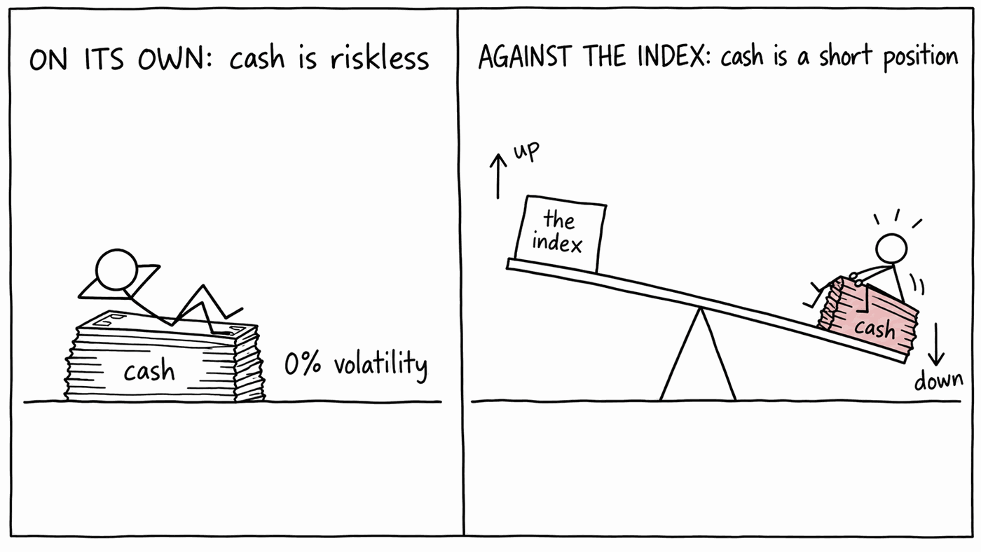
The plain covariance matrix does not show this, because it describes absolute returns, and in absolute terms cash really is riskless. A zero row in Σ forces a zero contribution no matter how large the active weight against it. The Euler identity still holds, so the contributions still sum to the tracking error and nothing looks obviously wrong, but the report attributes the risk to the wrong positions.
The fix: rotate the matrix into active space
Replace every covariance with the covariance of benchmark-relative returns:
You already have each piece:
- Cov(ri, rb) is the i-th element of
Σwb — one
MMULT. - Var(rb) is wb′Σwb, a single number.
Then decompose using your portfolio weights rather than your active weights, because the rotation has already removed the benchmark:
The total is identical, which is a good check on your algebra, and the attribution now falls on the positions that caused it. In the cash example, cash takes 100% and the stocks take 0%.
Two ways to build it
There are two routes to the rotated matrix, and they give identical numbers.
Route one: a relative returns tab. Work out the benchmark return for each week, subtract it from every stock return, and compute a covariance matrix of those relative returns exactly as you did in Module 3. Cash gets a column too: its relative return is simply the benchmark return with the sign flipped.
This is the more transparent route. Every number in the resulting matrix is something you can point at — the covariance between how much this stock beat the index and how much that one did. It is more work, but it is hard to get wrong.
Route two: adjust the matrix you already have. Take the absolute covariance matrix, subtract each stock's covariance with the benchmark along both the rows and the columns, then add back the benchmark variance. That is the formula above.
It is less typing, and frankly probably the easier route. But the adjustments are more abstract, and that makes it easier to make a mistake without noticing. It helps to recognise them as beta adjustments. The covariance of a stock with the benchmark is its beta times the benchmark variance, so
If you build both, subtract one matrix from the other. Every cell should be zero, and if it is, you can use either.
Route one: a relative returns tab
Put your benchmark weights in a row on a Weights sheet, in the same ticker
order as your returns. The benchmark return for each week is then:
=SUMPRODUCT(ReturnsW!B2:M2, Weights!$B$2:$M$2)RelW tab, with that benchmark return in column N, each stock:
=ReturnsW!B2 - $N2=-$N2RelW, cash column included. Only
the input has changed.
Route two: adjusting the matrix you already have
Add cash to your universe first: one extra row and column of zeros in the covariance matrix, a benchmark weight of 0, and a portfolio weight of 5%. Cash has zero absolute risk.
Then, beside your covariance matrix:
covib   =MMULT(Cov, wb)                        ' a column, one row per asset
varb =MMULT(TRANSPOSE(wb), MMULT(Cov, wb)) ' one cellcovib twice: once as a column down the side, and once transposed
as a row across the top. Each cell of the rotated matrix is then
=Cov!B2 - $M2 - N$1 + $O$1$M2 is that row's Cov(ri,rb), N$1 is that
column's, and $O$1 is Var(rb). Drag across and down.
On a 365 build, if covib is a spilled column you can do the whole thing in
one formula:
=Cov - covib - TRANSPOSE(covib) + varbTwo sanity checks before going further. The rotated matrix must still be
symmetric, and w_p' Sigma~ w_p must equal the tracking error you
already computed the ordinary way. If it does not, your row and column
vectors are the wrong way round.
Other cases
Cash is the simplest example, but the same problem arises whenever an asset's absolute risk is a poor guide to its benchmark-relative risk:
- Any holding that is not in the benchmark at all.
- A portfolio that is not fully invested, or is geared.
- A futures or derivative overlay, where notional and market value diverge.
- Any near-riskless asset: short-dated gilts, money market funds, collateral.
Wherever Σ has a small row and the active weight against it is not small, the naive decomposition will under-attribute risk to that position.
A caveat
The two decompositions answer different questions.
The naive one asks "if I scale this active position on its own, what happens to tracking error?" The rotated one asks "if I scale this holding, funded out of the benchmark, what happens?" The second matches what happens when you trade, which is why it is the better default.
You can see the difference without any cash at all. Take a portfolio with two stock tilts and everything else at benchmark weight. The naive decomposition gives exactly zero to every name held at benchmark weight. The rotated one does not, because in its counterfactual those holdings are funded against the index too — on our data they collectively carry about −0.5 percentage points of the tracking error.
Be clear which question you are answering. The main thing to avoid is using the naive decomposition on a portfolio that holds cash, where the largest active position disappears from the report.
Do both, and compare
Build the absolute decomposition and the active one side by side. The two rankings often differ noticeably, because an overweight in a low-volatility name can still be a large active bet.
Then add 5% cash to your own portfolio and run it both ways. The totals will agree; see where the attribution moves.
Check your answers
Sign in to get your own portfolio and have your answers marked.