Module 5 75 min

Time windows and exponential weighting

Your volatility estimate depends as much on the window you chose as on the market. Watch it move through 2008 and 2022.

Everything so far treated 2008 and last Tuesday as equally informative. This probably is not the case.

Choose your window

Take your portfolio and compute its annualised volatility over the full sample. Now recompute it using only the last 52 weeks. Then only the last 260.

The numbers will differ substantially — often by a factor of two.

Rolling windows

Put the window length in one cell, say Ctrl!B1 = 260, and the number of weekly observations in another:

Ctrl!B3   =COUNT(ReturnsW!B2:B1115)

which is 1,114. Then pick out the last N rows of your demeaned block with OFFSET:

=OFFSET(Dev!$B$2, Ctrl!$B$3 - Ctrl!$B$1, 0, Ctrl!$B$1, 81)

Feed that into the same MMULT(TRANSPOSE(...), ...) as Module 3, dividing by Ctrl!B1 - 1 rather than the full count. Typing a new window length then recalculates everything, so you can watch the answer change.

Count the data rows only. If your Dev sheet keeps the column means in row 1, as Module 3 suggests, then COUNT(Dev!B:B) picks those up too and every window ends one row past the end of your data.

OFFSET is volatile. The non-volatile equivalent joins two INDEX calls into a range:

=INDEX(Dev!$B$2:$CD$1115, Ctrl!$B$3 - Ctrl!$B$1 + 1, 0):INDEX(Dev!$B$2:$CD$1115, Ctrl!$B$3, 0)

Strictly, a window should be demeaned using the mean of that window rather than of the whole sample. Over 260 weeks the difference is small enough to ignore while you are exploring.

The trade-off

Short window. Picks up a change in conditions quickly. It is also noisy, and crises drop out of it quickly. A 52-week window in early 2007 had never heard of a financial crisis.
Long window. Stable, and keeps tail events in the estimate. It is also slow to react: in March 2020 a ten-year window was still mostly describing 2012.

Neither is right in general. The choice depends on which kind of error you would rather have, and it is worth stating which window you used.

Exponential weighting

Instead of a hard cut-off, where everything inside the window counts fully and everything outside counts zero, the weight on each observation can decay smoothly.

Σ = (1 − λ) Σ_k λ^k r_t−k r′_t−k

The most recent observation gets weight (1−λ), the one before λ(1−λ), and so on. The weights sum to one.

Half-life, the time until an observation counts half as much, is the easiest way to think about λ:

half-life = ln(0.5) / ln(λ)

λ	Half-life (daily)	Half-life (weekly)
0.94	11 days	11 weeks
0.97	23 days	23 weeks
0.99	69 days	69 weeks

λ = 0.94 is RiskMetrics' original daily parameter and has become a convention. It was fitted to 1990s data, so treat it as a starting point.

Building it in Excel

This looks harder than the sample covariance, but one rearrangement makes it straightforward.

You want a weighted sum of outer products. Scaling row t of your return matrix by √w_t and then forming R′R gives exactly that weighted sum, because each term of the product picks up √w_t twice.

So the recipe is:

Build a column of weights, oldest row first: =(1-lambda) * lambda^(n - ROW() + 1)
Normalise so they sum to 1: divide by their total.
Multiply each row of your returns by the square root of its weight. Use the raw weekly returns, not the demeaned ones from Module 3 — see the convention note below.
Run the same MMULT(TRANSPOSE(Rw), Rw) as Module 3 — with no division by T−1, because the weights already sum to one.

In practice

Weight column, with lambda in Ctrl!B2 and T rows of data:

=(1-Ctrl!$B$2) * Ctrl!$B$2^(Ctrl!$B$3 - (ROW()-1))

where Ctrl!B3 is the count of weekly observations, so the most recent row gets an exponent of zero. Then normalise. Scaled returns on a ScaledW sheet, with the weights in its column A:

=ReturnsW!B2 * SQRT($A2)

And the matrix:

=MMULT(TRANSPOSE(ScaledW!B2:CD1115), ScaledW!B2:CD1115)

Changing λ in one cell then updates the whole model.

A convention you should know

RiskMetrics does not demean returns before computing EWMA covariance: it assumes the mean is zero. At daily and weekly frequency the mean is tiny relative to the volatility, and not estimating it removes a source of noise. Our answer key follows that convention, which is why the recipe above uses raw returns. On this data demeaning first moves the answer by up to about 1.3% — inside the checker tolerance, but closer to the edge than you want, so if an EWMA check is refusing you, that is the first thing to look at.

Watching it through the crises

Compute your portfolio's EWMA volatility at each week-end through the sample and chart it. Overlay a rolling 104-week sample volatility.

You should see:

September 2008. EWMA vaults upward within weeks. The rolling window climbs slowly, because four years of calm are still in it.
2009–2010. EWMA falls back quickly as markets settle. The rolling window stays elevated for much longer, because 2008 is still inside it.
March 2020. The sharpest move in the sample. EWMA(0.94) roughly doubles in a month.
September 2022. The gilt and LDI crisis, which is particularly relevant given where you work. Aggregate equity volatility barely moved: EWMA(0.94) averaged 15.1% over September and October, against 14.8% for a rolling 104-week window. The stress was concentrated in the gilt market.

The sector detail shows where it did appear. Daily volatility in those two months, as a multiple of the same names' calm-2022 volatility:

Industry Multiple

Real Estate 1.60

Utilities 1.25

Financials 0.99

Basic Materials 0.90

Energy 0.74

The effect was concentrated in rate-sensitive sectors. Real estate and utilities are long-duration assets that behave partly like bonds, and the move in gilt yields repriced them. Banks, which earn more as rates rise, barely moved. It is a useful reminder to ask how a shock is transmitted before assuming which sectors it will affect.
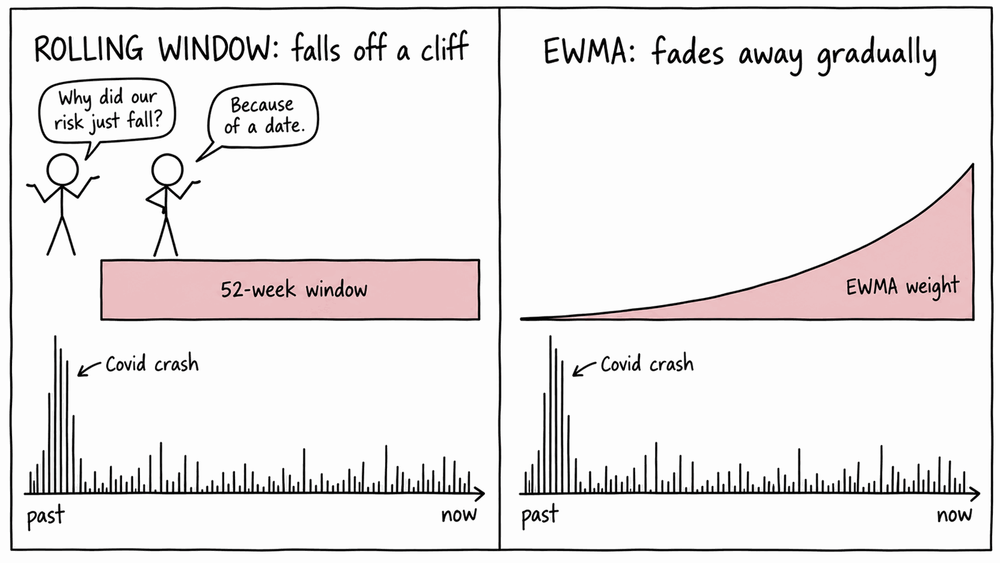
The one-year anniversary problem. Watch a rolling 52-week estimate through early 2021. On 24 February it reads 34.5%; five weeks later, on 31 March, it reads 21.1%. The drop is caused by the Covid crash leaving the window.

EWMA(0.94) over the same weeks goes from 21.8% to 18.8%, a fall of 3 points compared with 13.

This causes practical problems: the number moves, a portfolio manager asks why, and the honest answer is "because of a date". It helps to be able to explain this, and to have the EWMA comparison to hand.

Industry	Multiple
Real Estate	1.60
Utilities	1.25
Financials	0.99
Basic Materials	0.90
Energy	0.74

EWMA avoids this, because old observations fade gradually instead of falling off a ledge. That is one of the main reasons to use it.

Two cartoon panels, each showing weekly returns as spikes along a timeline from past to now, with a cluster of very tall spikes near the start labelled Covid crash. Left, titled Rolling window: falls off a cliff. A flat pink block labelled 52-week window starts just after the Covid spikes, leaving them outside; one stick figure asks Why did our risk just fall? and another answers Because of a date. Right, titled EWMA: fades away gradually. A pink curve labelled EWMA weight rises smoothly from almost nothing over the Covid spikes to its peak at now. — A rolling window gives every week inside it full weight and every week outside it none, so a crisis leaves all at once. EWMA's weights shrink smoothly, so the same crisis fades out over time.

What to take away

Always state the window when you quote a volatility.
Short windows react; long windows remember.
EWMA responds quickly without the anniversary effect.
λ = 0.94 is a convention, and you can change it.

Check your answers

← Tracking error and where the risk comes from

Value at Risk →