Skew, kurtosis, and a VaR that believes them
Measure how far returns are from normal, watch the measurement wobble when you change the sampling day, then feed it into a VaR.
Module 6 found historical VaR coming out above parametric VaR, and put the gap down to the fat left tail of equity returns. This module measures that tail directly, then tries to put the measurement back into a VaR number.
Volatility is the second moment of the return distribution. The next two moments describe its shape.
The third and fourth moments
With weekly returns r, their mean r̄ and standard deviation s:
- Skew measures lopsidedness. Cubing keeps the sign, so large falls push it negative and large rises push it positive. A normal distribution has a skew of zero.
- Kurtosis measures how much of the variance comes from rare, extreme observations. The fourth power makes every sign positive and makes big numbers enormous: a 5-sd week contributes 625 to the sum, and a 1-sd week contributes 1. A normal distribution has a kurtosis of exactly 3, so people usually subtract the 3 and quote excess kurtosis, which is zero for a normal.
Doing it in Excel
With your weekly portfolio returns in PortRet, as in Module 6:
=SKEW(PortRet)
=KURT(PortRet)
KURT already subtracts the 3, so it returns excess kurtosis. Some
textbooks and some software quote raw kurtosis, where a normal distribution
scores 3. Check which one you are looking at before you compare numbers:
on these portfolios an extra 3 typically makes the answer about half as big
again.
Both functions use small-sample corrections, like STDEV.S. SKEW.P exists
if you want the population version; there is no KURT.P. With 1,114
observations the corrections are tiny: on our portfolios the population
formulas above differ from SKEW by about 0.1% and from KURT by about
0.6%, both well inside the checker's tolerance.
What the benchmark looks like
The CAPFIXED_TR benchmark, sampled Wednesday to Wednesday, gives 1,114 weekly
returns with a weekly standard deviation of 2.37%, a skew of −0.47 and
an excess kurtosis of 5.64.
Those numbers are easier to feel as a count of extreme weeks:
| Weeks below | Weeks above | A normal distribution expects, each side | |
|---|---|---|---|
| Beyond 3 sd | 11 | 9 | 1.5 |
| Beyond 4 sd | 5 | 3 | 0.04 |
The worst week, to 18 March 2020, was −13.9%: 5.9 standard deviations. A normal distribution expects a week like that about once every 13 million years. It turned up in March 2020.
The negative skew shows in the rows as well: more of the extreme weeks are falls than rises. That pattern holds for joiners' portfolios too. Of 300 portfolios built the same way as yours, 98% have negative skew.
Change the day, change the kurtosis
Now do something that ought to make no difference. Sample the same benchmark on
each day of the week in turn, using the Module 2 routine with a different
WEEKDAY value, and recompute:
| Sampled on | Skew | Excess kurtosis | Annualised vol |
|---|---|---|---|
| Monday | −0.25 | 5.68 | 17.86% |
| Tuesday | +0.02 | 7.51 | 16.91% |
| Wednesday | −0.47 | 5.64 | 17.11% |
| Thursday | −0.88 | 9.06 | 17.32% |
| Friday | −0.85 | 10.49 | 17.77% |
Volatility moves by about 5% from the lowest to the highest. Kurtosis nearly doubles, from 5.64 to 10.49, and on Tuesdays the skew changes sign. Same companies, same prices, same twenty-one years.
Why it happens
A crash rarely happens in a single day. It runs across several, and whether a weekly return captures it depends on where the week boundary falls. Here is the worst stretch of October 2008, day by day:
| Mon 6 | Tue 7 | Wed 8 | Thu 9 | Fri 10 | Mon 13 |
|---|---|---|---|---|---|
| −7.6% | −0.2% | −5.7% | −1.2% | −9.1% | +7.5% |
And the same fortnight as weekly returns:
| Sampled on | The two weeks |
|---|---|
| Friday | −21.8%, then +2.5%: the whole collapse lands in one week |
| Wednesday | −12.4%, then −6.8%: split down the middle |
| Monday | −3.5%, then −9.0%: split, and the Monday rebound cancels part of it |
Friday sampling turns five bad days into one gigantic observation. Wednesday turns them into two large ones. Raised to the fourth power, one −21.8% week counts for far more than two moderate ones, so the Friday kurtosis goes up and the Wednesday one does not.
Three weeks out of 1,114
Drop the three most extreme weeks from each series and recompute. The spread in kurtosis across the five weekdays shrinks from 4.85 to 1.29. Most of the disagreement rests on three observations.
That is because a handful of weeks supply most of the fourth moment. On Wednesdays, the three biggest weeks, all from March 2020, account for a third of the whole sum of fourth powers, and the ten biggest account for 65%. On Fridays the top three account for 60%.
So a kurtosis estimate is mostly a report on a few crisis weeks, and on exactly where the sampling grid happened to cut them.
So is Wednesday the wrong day?
Module 2 chose Wednesday because it avoids stale prices on bank holidays, which matters for volatility, and that reason still stands. No day gives the "right" kurtosis: each one just cuts the crises in different places.
Nor is there a tidy link between holidays and kurtosis. Monday sampling hits a closed market most often, 106 times, and has one of the lowest kurtosis figures.
Try it on your own portfolio
Compute the skew and excess kurtosis of your portfolio's Wednesday returns, then resample on Fridays and compute them again. Across our 300 portfolios, Friday kurtosis came out higher in 84% of cases, by a median of 37%.
Cornish–Fisher VaR
Parametric VaR in Module 6 assumed a normal distribution and used z = −2.326 for the 99th percentile. The Cornish–Fisher expansion adjusts that quantile for skew S and excess kurtosis K:
With S and K both zero it collapses back to the normal quantile, so everything from Module 6 carries over and this is one extra layer on top.
Doing it in Excel
S       =SKEW(PortRet)
K       =KURT(PortRet)
z       =NORM.S.INV(0.01)
z_cf    =z + (z^2-1)*S/6 + (z^3-3*z)*K/24 - (2*z^3-5*z)*S^2/36
CF VaR =-z_cf * STDEV.S(PortRet)On the Wednesday benchmark the terms come out as:
| Term | Value |
|---|---|
| Normal quantile, z | −2.326 |
| Skew adjustment | −0.348 |
| Kurtosis adjustment | −1.319 |
| Skew-squared correction | +0.084 |
| zcf | −3.908 |
The kurtosis term does most of the work. It moves the quantile out by 1.3 standard deviations, more than half the size of the normal quantile itself.
A gotcha: at 95%, fat tails make VaR smaller
A question worth trying on a colleague. Equity returns have fat tails. Is their 95% VaR higher or lower than a normal distribution with the same volatility would give?
Most people say higher, since VaR is a tail measure and the tails are fat. At 95% it is usually lower.
The kurtosis term shows why. Its coefficient, (z³ − 3z)/24, changes sign at z = −√3, which is the 95.8% confidence level:
| Confidence | z | Effect of each point of excess kurtosis on z |
|---|---|---|
| 95% | −1.645 | +0.020, pulling the quantile in towards zero |
| 99% | −2.326 | −0.234, pushing it out |
This is what fat tails mean once the volatility is held fixed. A fat-tailed distribution has more weight in its peak and more in its far tails, and with the same variance that weight has to come from somewhere: the shoulders, roughly one to two standard deviations out. The 95% point, at 1.645 standard deviations, sits in the shoulder. Fewer than 5% of weeks land beyond it, so the real 95% loss is closer to zero than the normal one.
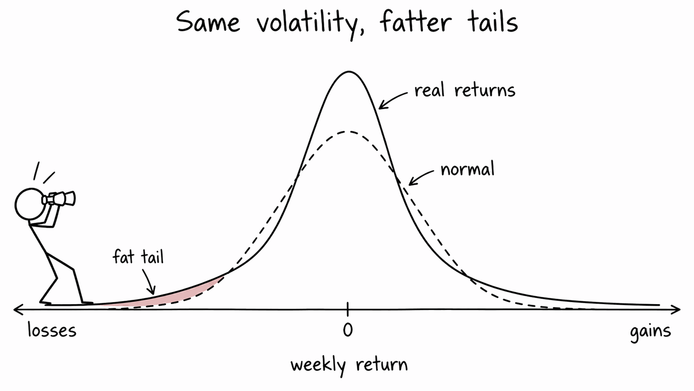
The data agrees. On the Wednesday benchmark, with Module 6's parametric and historical VaR at several confidence levels:
| Confidence | Parametric | Historical | Weeks worse than parametric | A calibrated model expects |
|---|---|---|---|---|
| 90% | 3.04% | 2.37% | 73 | 111 |
| 95% | 3.90% | 3.44% | 45 | 56 |
| 97.5% | 4.65% | 4.98% | 34 | 28 |
| 99% | 5.52% | 6.82% | 21 | 11 |
| 99.5% | 6.11% | 8.05% | 18 | 6 |
Up to 95% the normal distribution is too cautious. By 97.5% it is not cautious enough, and the further out you go the worse it gets.
Some of the gap at 95% comes from the mean, rather than the shape. Historical VaR uses the actual returns, which averaged +0.19% a week, while parametric VaR assumes a mean of zero. Subtract the mean from each return first and historical 95% VaR rises from 3.44% to 3.63%, still below the parametric 3.90%. On those demeaned returns the two measures cross at 96.4%.
It is not a quirk of the benchmark. Across 300 portfolios built the same way as yours:
- At 95%, historical VaR was below parametric in all 300, by a median of 11%. On demeaned returns it was still below in 94% of them, by a median of 6%.
- At 99%, historical VaR was above parametric in all 300.
- The crossover sat at a median of 96.4%, and between 95.4% and 97.3% for four portfolios in five. Like everything else in this module it moves with the sampling day: from 94.5% on Tuesdays to 97.4% on Fridays, for the benchmark.
Why it matters
95% is a common confidence level for internal risk reporting, and it was the original RiskMetrics convention. Someone who warns that fat tails mean a 95% VaR is understated has it the wrong way round for that number. The fat-tail warning belongs to 99% and beyond, and to expected shortfall, which averages over the whole tail.
Compute your own portfolio's 95% historical VaR, and the 95% parametric VaR alongside it, and see which side of the line it falls.
It overshoots
Put the result next to the Module 6 numbers, for the same benchmark:
| One-week 99% | |
|---|---|
| Parametric VaR | 5.52% |
| Historical VaR | 6.82% |
| Cornish–Fisher VaR | 9.28% |
| Historical expected shortfall | 9.53% |
You might expect a normal VaR adjusted for fat tails to land somewhere between the normal answer and the historical one. It lands well beyond both. That was not a fluke of the benchmark: across the 300 portfolios, Cornish–Fisher VaR was above historical VaR every single time, by a median of 37%.
It lands close to expected shortfall instead: a median of 0.99× ES, with the middle half of portfolios between 0.93 and 1.06. Nothing in the formula promises that, so treat it as a curiosity of this dataset and do not lean on it.
The reason for the overshoot is that the expansion is a series approximation around the normal distribution, and it works best for mild departures from it. An excess kurtosis of 5.6 is not mild. The kurtosis term grows in a straight line with K, and at the 99% level every extra point of K pushes the quantile out by another 0.23 standard deviations.
Count exceptions over the whole sample, as in Module 6. On the Wednesday benchmark you would expect about 11:
| VaR used | Weeks worse than it |
|---|---|
| Parametric | 21 |
| Historical | 12 |
| Cornish–Fisher | 5 |
Parametric is breached twice as often as it should be; Cornish–Fisher less than half as often. Historical scores well, but remember Module 10: it was estimated on these very weeks, so it is guaranteed to get close.
And it moves with the weekday
Because Cornish–Fisher VaR is built on kurtosis, it inherits kurtosis's sensitivity to the sampling day. On the benchmark, moving from Wednesday to Friday sampling:
| One-week 99% | Wednesday | Friday | Change |
|---|---|---|---|
| Parametric VaR | 5.52% | 5.73% | +4% |
| Historical VaR | 6.82% | 6.52% | −4% |
| Cornish–Fisher VaR | 9.28% | 12.64% | +36% |
Across the 300 portfolios the Friday Cornish–Fisher VaR was a median 16% higher than the Wednesday one, against 3% for historical VaR.
When the expansion stops being a distribution
An adjusted quantile has to go up as the probability goes up, or it does not describe a distribution at all. With Friday's excess kurtosis of 10.5 the Cornish–Fisher curve fails that test: between about −0.3 and +0.55 on the normal scale it runs backwards. That stretch is in the middle of the distribution rather than the tail, so the 99% number still computes, but it is a clear sign that the correction is being asked to do more than it can.
So the question from Module 6 comes back sharper. A risk number that jumps by a third when you change the day of the week you sample on is telling you more about three weeks in 2008 and 2020 than about next week. Module 12 stops summarising the tail with moments and looks at the tail itself.
What to take away
- Skew and kurtosis describe the shape of the distribution; equity returns have negative skew and fat tails.
- Kurtosis is dominated by a few extreme weeks, so it depends heavily on how those weeks are sampled.
- Fat tails raise VaR only far out. Below about 96% confidence the normal distribution gives the larger number.
- Cornish–Fisher VaR corrects the normal quantile using those moments. On this data it overshoots historical VaR, and it inherits all of kurtosis's instability.
- Before trusting a number built on the fourth moment, change the sampling day and see whether it survives.
Check your answers
Sign in to get your own portfolio and have your answers marked.